Computer vision digitization of smartphone images of anesthesia paper health records from low-middle income countries | BMC Bioinformatics

The extraction of data from an anesthesia paper chart begins with optimizing the lighting of the smartphone photographs, removing shadows, and using object detection to find document landmarks for use in removing perspective distortion. Then, each section of the chart is identified by a YOLOv8 model and cropped out of the chart. YOLOv8 models which are trained to detect handwritten blood pressure symbols, numbers, and checkboxes used in anesthesia paper charts produce lists of bounding boxes that a combination of convolutional neural networks, traditional computer vision, machine learning, and algorithms then use to impute meaningful values and detect errors.

Image optimization techniques

To maximize the accuracy of digitization, the input images need to be optimized as follows: (1) shadows removed, (2) pixel intensities standardized and normalized, (3) perspective distortions such as rotation, shear, and scaling corrected, and (4) general location of document landmarks fixed. We accomplish this by first removing shadows using image morphology techniques, then normalize and standardize the pixel values of the images, and finally correct perspective distortions and approximately correct the location of document landmarks using a homography transformation.

Shadow removal

Smartphone photographs of the anesthesia paper chart often suffer from sudden changes in pixel intensities caused by shadows being cast onto the image which break up the lighting. Sudden changes in the value of pixels can cause difficulty for deep learning models which learn representations of objects as functions of the weighted sums of pixels. Therefore, both normalization and shadow removal are necessary to optimize our inputs and maximize detection accuracy. One algorithm for accomplishing this is outlined by Dan Mašek in a stack overflow post from 2017 (Algorithm 1) [10].

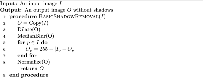
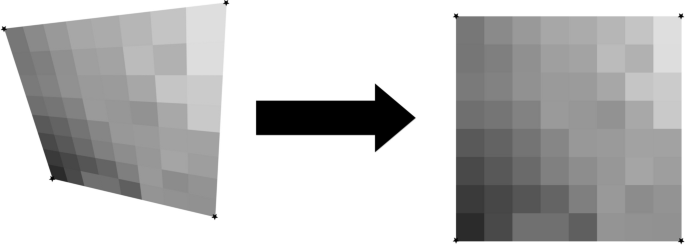
The exact values for the median blur and dilation operations are subject to the image’s size and degree of shadow and can be tuned to the dataset. This algorithm only operates on grayscale images, but since no information in the anesthesia paper charts are encoded with color, we converted our charts to grayscale. We did not use any metrics to assess shadow removal, but a visual inspection of the output shows that the resulting images no longer suffer from a lighting gradient (Fig. 2).

Example of an anesthesia paper chart before and after the removal of shadows and normalization. The dilated, blurred image is subtracted pixel-wise from the original image to produce the final result

The planar homography

The planar homography is defined as the most general linear mapping of all the points contained within one quadrilateral to the points of another quadrilateral (Fig. 3). A planar homography was used to correct perspective distortions within the smartphone image.

An illustration of a homography performing a general linear mapping of the points of one quadrilateral to another. Images suffering from perspective distortions can have much of their error corrected by finding four anchor points on the image, and using them as the four points on a quadrilateral to map to a perfect, scanned sheet

Translation, rotation, scaling, affine, and shear transformations are all subsets of the homography, and the homography in turn can be decomposed into these transformations. Here, as in many other computer vision applications, the homography is used to correct linear distortions in the image caused by an off-angle camera perspective (Fig. 4).

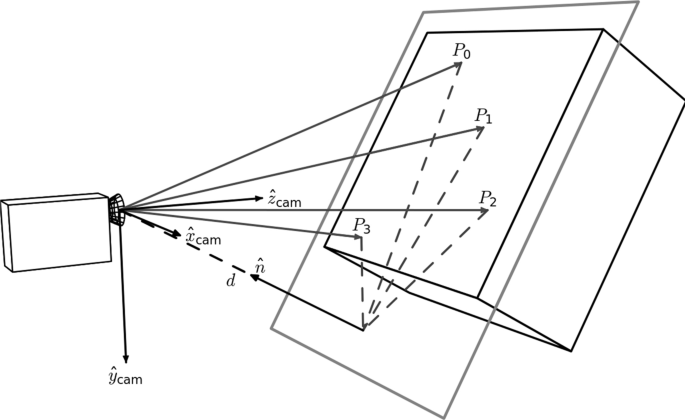
An illustration of perspective based distortion due to an off-angle camera. Even the most vigilant camera operators will have some degree of perspective distortion. [11]

In order to compute a useful homography for document correction, four document landmarks need to be identified from a target anesthesia paper chart image. Those same four landmark locations were then identified on a scanned, perfectly aligned control anesthesia paper chart image. We trained a YOLOv8 model to detect the document landmarks “Total”, “Time”, “Procedure Details”, and “Patient Position” which fall in the four corners of the anesthesia paper chart described in Fig. 1. We then used the OpenCV python package to compute the homography between the two sheets and warp the target image accordingly (Fig. 5). The benefits to this method are that the homography computation is robust to failure due to YOLOv8’s high accuracy, even under sub-optimal conditions. In cases where the planar homography failed to correct the distortion, clear errors were found on the anesthesia paper chart including: (1) landmarks being obscured by writing (2) landmarks being covered by other pieces of paper (3) landmarks not being included in the smartphone image entirely. Initially, this deep object detection approach seems excessive, as there are a number of traditional computer vision methods for automatic feature matching between two images such as ORB and SIFT. However, the variance in lighting and blurriness in our dataset posed challenges for these nondeep algorithms, which often failed silently, mistaking one landmark for another, and warping images such that they were unidentifiable.

An illustration of correction using a homography on an image of the anesthesia paper chart. Perspective based distortions are corrected

Section extraction

There are seven sections which encode different pieces of intraoperative information on the anesthesia paper chart (Fig. 1). Due to nonlinear distortions in the image, the homography is not a perfect pixel-to-pixel matching from the target image to the scanned control image. Therefore, an alternative method of identifying the precise location of the sections is required. We accomplished this by training a YOLOv8s model to place a bounding box around each section. Because the homography already normalizes the locations of the sections to within a few dozen pixels, we were able to train one of the smallest architectures of YOLOv8, YOLOv8s, to extract the different sections.

Image tiling for small object detection

The anesthesia paper chart is characterized by having handwritten symbols (e.g., medication, numerical and blood pressure symbols) that are small and often tightly packed together (Fig. 1). Single shot detectors like YOLO struggle to separate and identify these handwritten symbols due to their use of a grid which assigns responsibility of a single cell to the center of a single object. One solution to this issue is to increase the image size, however since YOLO uses padding to make all images square, and the number of pixels in a square image grows quadratically with image size, this causes training memory usage and detection time to increase quadratically as well. To overcome this problem, we used an approach called image tiling where we divided the image into smaller pieces called tiles and trained on the tiles rather than the entire image. This allowed us to increase the size of these small objects relative to the frame, allowing us to get much better object detections.

There are, however, several challenges associated with image tiling. First, objects which are larger than the tiles which we have divided the image into will not be able to fit into a single tile, and will be missed by the model. All the handwritten symbols in our dataset were small, and were uniform in size, allowing us to use image tiling without the risk of losing any detections. Second, by needing to detect on every sub-image, the detection time increases. Whereas this may be an issue in real-time detection, the difference in detection time is only measured in several hundred milliseconds, which does not affect our use case. Third, the number of unique images and total objects in a single training batch will be smaller, causing the models weights to have noisy updates and require longer training. We solved these issues by utilizing the memory savings acquired by tiling to double the training batch size from 16 to 32. In addition, due to the very large number of empty tiles, we were able to randomly add only a small proportion to the training dataset, which further increased the object to tile ratio. Finally, objects which lie on the border of two tiles will not be detected since they do not reside in either image. Our solution to this issue is to not divide the image into a strict grid, but instead to treat the tiling process as a sliding window which moves by one half of its width or height every step. With this approach, if an object is on the edge of one sub-image, it will be directly in the center of the next one (Fig. 6). This solution introduces its own challenge though since nearly every detection will be double counted when the detections are reassembled. Our solution to this problem is to compute the intersection-over-union of every bounding box with every other bounding box at detection time, group together boxes whose intersection-over-union is greater than a given threshold, and combine them into one detection. Since the objects we are detecting should be well separated and never overlap, this allows us to remove the doubled detections.

An example of our implementation of image tiling. By using a sliding window rather than a grid, the edge of one image is the center of the next one [12]

Blood pressure symbol detection and interpretation

The blood pressure section encodes blood pressure values using arrows, and heart rate using dots or lines. Each vertical line on the grid indicates a five minute epoch of time during which a provider records a blood pressure and heart rate reading (Fig. 1). The y-axis encodes the value of blood pressure in mmHg, and each horizontal line denotes a multiple of ten (Fig. 1).

Symbol detection

Systolic blood pressure values are encoded by a downward arrow, and diastolic blood pressure values are encoded with an upward arrow. The downward and upward arrows are identical when reflected over the x-axis, so we were able to collapse the two classes into one. We then trained a YOLOv8 model on the single “arrow” class, and during detection we simply detect on the image and an upside-down-version of itself to obtain systolic and diastolic detections respectively. Finally, the  diastolic detections y-values are subtracted from the image’s height to correct for the flip.

Thereafter two key pieces of information are required from each of the bounding boxes: (1) its value in millimeters of mercury (mmHg), and (2) its timestamp in minutes.

Inferring mmHg values from blood pressure symbol detections

The value of blood pressure encoded by an arrow corresponds to the y-pixel of the tip of the arrow. By associating a blood pressure value to each y-pixel in the blood pressure section, we can obtain a value for each blood pressure bounding box. We trained a YOLOv8 model to identify the 200 and 30 legend markers, and by identifying the locations of the 200 and 30 markers, we were able to interpolate the value of blood pressure for each y-pixel between the 200 and 30 bounding boxes (Fig. 7).

By dividing the space between the 30 and 200 bounding boxes equally, we can find the blood pressure values of each y-pixel. We ran the algorithm on this image, and set all the y-pixels that were multiples of 10 to red. We can see the efficacy of the algorithm visually as the detections cover the lines on the image almost perfectly

Assigning timestamps to blood pressure symbol detections

To impute timestamps, we wrote an algorithm that applies timestamps based on the relative x distances between the systolic and diastolic detections (algorithm 2).

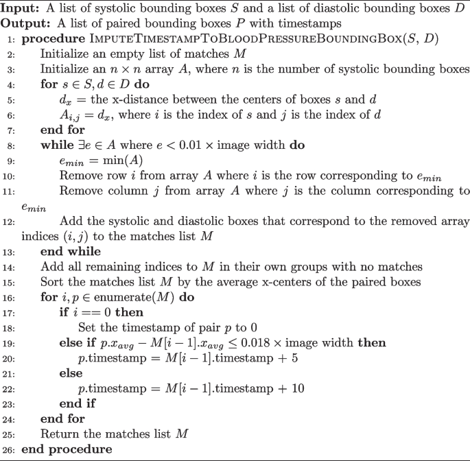
Imputing a Time Stamp to a Blood Pressure Bounding Box

Missing detections are a common problem when applying timestamps. Our algorithm deals with this in two ways. The while loop checks if two boxes are within 1% of the image’s width from one another, ensuring they are not too far away to plausibly match before actually pairing them. If a box has no pair which is within the 1% range, the algorithm considers it to not have any matches. Another problem occurs when there are no detections for a five minute epoch. This is solved by sampling the distance between true matches in the dataset. We found that 100% of the matches were within 0.016*image’s width of the next matching pair. So, adding a small amount for error, if a match is more than 0.018*image’s width from the next pair, a time gap of 10 min is applied instead of the typical 5.

Blood pressure model training and error testing

A YOLOv8l model, the second largest architecture of YOLOv8, was trained to detect downward arrows for 150 epochs and using a batch size of 32 images. The images used to train this model were tiled images of the blood pressure section where only the systolic arrows were annotated on unflipped images, and only the diastolic arrows were annotated on flipped images.

There are two ways that error will be assessed for the blood pressure section: detection error and inference error. Detection error will be computed using the normal object detection model metrics of accuracy, recall, precision, and F1. Inference error is the error between the value in millimeters of mercury the program assigned to a blood pressure detection on the whole image of the blood pressure section, and the ground truth value that was manually annotated. Blood pressure detections made by the program were hand matched with ground truth values during assessment in order to avoid the case where the correct blood pressure value was assigned to a different timestamp. The error metric we used for this was mean average error. The 30 chart images used for testing included 1040 systolic and diastolic marks (this number varies from the object detection testing set due to image tiling duplicating detections). The ability of the program to match blood pressure detections to a particular time stamp was not assessed.

Physiological indicators

The physiological indicators section is the most difficult and challenging section to digitize. Handwritten digits are written on the line that corresponds to the physiological data they encode, but are free to vary along the time axis rather than being discretely boxed in, or being listed in fixed increments. In addition, the individual digits which appear in the physiological indicators section must be concatenated into strings of digits to form the number the provider intended to write. Our approach to digitize this section is described below:

Handwritten number detection

Our approach for the detection of numbers is a two-step process: (1) a YOLOv8 model trained on a single “digit” class which locates and bounds handwritten numbers, and (2) a RegNetY_1.6gf CNN that classifies those digits. There are two advantages to this method over using a single YOLOv8 model for both detection and classification. First, the distribution of digits in our training dataset was not uniform. For example, there are over one-thousand examples of the number ’9’ on the training charts, but only approximately 160 examples of the number ’5’ due to the typical range of oxygen saturation being between 90 and 99. This leads to the number 5 having much poorer box recall in a model that does both classification and localization. Visually, handwritten numbers are very similar to one another, so by collapsing each digit into a single “digit” class, the model can learn information about how to localize handwritten digits for numbers which are underrepresented by using numbers which are overrepresented. Second, there is an added advantage of training the classification CNN separately since the dataset can be augmented with images of digits not found on the anesthesia paper charts. We used the MNIST dataset to expand and augment our training dataset, providing sufficient examples from each class to attain a high accuracy [13].

Matching each box to the corresponding row

Prior to clustering the digit bounding boxes together by proximity (Fig. 9), we had to find which row the box belongs to. For any given patient, between 0 and 7 rows were filled out depending on the type of surgery and ventilation parameter data recorded by the anesthesia provider. For the special cases where 0 or 1 rows were filled out, there were either no detected digits or the standard deviation of the y-center of the detected digits was only a few pixels. For the case where there was more than one row, we used KMeans clustering on the y-centers of the digit bounding boxes using \(k \in [2, 3, 4, 5, 6, 7]\) and determined the number of rows by choosing the value of k which maximized the silhouette score, a metric which determines how well a particular clustering fits the data. In order to determine which row a cluster encodes, we examined the y-centroid of clusters from 30 sheets, and found that the distribution of y-centroids for a particular row never overlapped with any other row. This meant that there were distinct ranges of y-pixels that corresponded to a given row, allowing us to determine which row a cluster encodes by finding which range contained the y-centroid of a cluster (Fig. 8).

Clustered detections in the physiological indicator section using the KMeans clustering algorithm, and selecting K based on the maximum silhouette score

Clustering single digit detections into multi-digit detections

When we assigned each row an ordered list of boxes that correspond to it, we then clustered those boxes into observations that encode a single value (Fig. 9). This is done with the same KMeans-silhouette method used to find which rows each digit bounding box corresponds. In order to narrow down the search for the correct value of k, we used the plausible range of values for each row. For example, the first row encodes oxygen saturation, which realistically falls within the range \(\text SpO_2 \in [75, 100]\). If we let n be the number of digit bounding boxes, the minimum number of clusters would be realized if the patient had a \(100\%\) oxygen saturation for the entire surgery, leading to \(k = \lfloor n/3\rfloor\). In contrast, the maximum number would be realized when the patient never had a \(100\%\) oxygen saturation, leading to \(k = \lceil n/2\rceil\). Allowing for a margin of error on either side of \(10\%\) due to missed or erroneous detections, we fit a KMeans clustering model with each of \(k \in [\lfloor n/3\rfloor – \lceil 0.1*n \rceil , \lceil n/2\rceil + \lceil 0.1*n\rceil ]\), and selected the value of k which maximized silhouette score. For the other physiological parameter rows, we reassessed the plausible number of digits for that specific variable and obtained a new range of k values. The clusters created by the optimal KMeans model are then considered to be digits which semantically combine to form one value.

Boxes from the SpO₂section clustered into observations using KMeans. A plausible range of values for k is determined by computing the number of boxes divided by the highest and lowest plausible number of digits found in a cluster (3 and 2 for the SpO₂ section, respectively). From this range, the k which maximizes the silhouette score is chosen

The only section which does not conform to this paradigm is the tidal volume row. In this row, there is an “X” which separates a tidal volume in milliliters from the respiratory rate in breaths per minute. To detect semantic groupings of digits, we used the fact that tidal volume is nearly always three digits, and respiratory rate is nearly always two digits, with an “X” mark in the center, and made our search accordingly. A small CNN trained as a one vs rest model to detect the “X” mark was then trained to separate the tidal volume from the respiratory rate.

Assigning a value to each multi-digit detection cluster

We trained a RegNetY CNN model to classify images of handwritten numbers by combining the MNIST dataset with the digits from the charts we labeled. Initially the program runs the model on each digit in a cluster and concatenates them together to form a single value. However, due to the poor quality of handwriting, our test set classification accuracy was approximately 90% rather than the standard 99% or greater that is achievable with most modern CNNs using the MNIST dataset.

One way to minimize this error is to check if the value assigned is biologically plausible. The program first checks if the concatenated characters of a section fall in a plausible range for each row. For example, if SpO₂\(\not \in [75\%, 100\%]\) the program marks the observation as implausible. In addition, if the absolute difference between a value and the values immediately before or after it is larger than a one sided tolerance interval constructed with the differences we observed in the dataset, the program also marks it as implausible. For example, if an observation for SpO₂ is truly 99, but the model mistakes it is 79, and the observations just before and after it is 98 and 100 respectively, the observation is marked as implausible since SpO₂ is very unlikely to decrease and improve that rapidly. If an observation is marked as implausible, the program imputes a value by fitting a linear regression line with the previous two and next two plausible values, and predicts the current value by rounding the output of the regression model at the unknown value.

Physiological indicator model and error testing

A YOLOv8l model was trained to detect one class, handwritten digits, for 150 epochs with a batch size of 32.

A RegNetY_1.6gf model was trained on a mixture between observations cropped from the charts and the MNIST dataset. The model was validated and tested on observations only from the charts. The training set contained 88571 observations, while the validation and testing sets had 7143 observations each. The model was trained for 25 epochs and images were augmented using Torchvision’s autoaugment transformation under the ’imagenet’ autoaugment policy.

Error for object detection will be assessed with accuracy, precision, recall, and F1. Error for classifying numbers will be reported using only accuracy. The error for inferring a value from the classified object detections will be assessed using mean average error on each of the 5 physiological indicators on all 30 test charts. Using the output of the program and the ground truth dataset, we will compute the mean average error by index value of the lists. For example, let the program output be (99, 98, 97), the ground truth from the chart image be (98, 99, 100). Then the matched values are ((99, 98), (98, 99), (97, 100)), and the error would be computed as \(((\Vert 99-98\Vert + \Vert 98-99\Vert + \Vert 97-100\Vert )/3))\). If the ground truth and predictions vary in length, the longer of the two lists will be truncated to the length of the shorter.

Checkboxes

The checkbox section is a two class object detection and classification problem. Imputing a value can be made difficult if there are missing or erroneous detections.

Checkbox detection and classification

We labeled each checkbox from all the anesthesia paper charts in the dataset as checked or unchecked, and then trained a YOLOv8 model to detect and classify each checkbox in the image. Approximately one out of every twenty checkboxes that were intended to be checked did not actually contain a marking inside them. Instead, the marking would be placed on the text next to the box, slightly above the box, or adjacent to the box in some other location. We decided a priori to label these as checked because it was the intention of the provider to indicate the box as checked, and so that the model would begin to look to areas adjacent to the box for checks as well.

Assigning meaning to checkboxes

The checkboxes are arranged in columns (Fig. 1), so the algorithm for determining which bounding box corresponds to which checkbox starts by sorting the bounding boxes by x-center, then groups them using the columns that appear on the page, and sorts each group by y-center. For example, the left-most boxes “Eye Protection”, “Warming”, “TED Stockings”, and “Safety Checklist” on the anesthesia paper chart are all in the “Patient Safety” column, and have approximately the same x-center. The algorithm sorts all checkbox bounding boxes by x-center, selects the first four, then sorts them by y-value. Assuming there are no missing or erroneous boxes, these first four bounding boxes should match the “Patient Safety” checkboxes they encode.

Checkbox model training and error testing

A YOLOv8l model was trained to detect and classify checkboxes for 150 epochs using a batch size of 32. Error will be reported by overall accuracy, precision, recall, and F1 score. Sheets where the number of detections does not match the number of checkboxes will be removed from the error calculation, and the number of sheets where this occurred will be reported.

In addition to detection and classification, the program’s ability to correctly infer which checked/unchecked bounding box detection associates with which checkbox will be assessed. This error will be quantified with accuracy, precision, recall, and F1.